Modeling Credit Risk in Mortgage Lending: Estimating Probability of Default

Modeling Credit Risk

Prior to the Great Financial Crisis (GFC) in 2008, credit rating agencies, such as Moody’s, assigned high credit ratings to mortgage obligors. This resulted in over half of their structured finance securities receiving AAA ratings. These high ratings were driven by profit, given that large investment banks were restricted to investing solely in triple A-rated securities. However, by the end of 2007 and the beginning of 2008, only 33% of these triple A-rated securities kept their ratings after downgrading, leading to the fragility of the financial system (Benmelech & Dlugosz, 2010). In response to the GFC, the Basel Committee introduced Basel III, which offers various credit risk approaches, including Foundation Internal Ratings-Based (F-IRB) and Advanced Internal Ratings-Based (A-IRB) methods. In these approaches, financial institutions can estimate their own Probability of Default (PD), the likelihood that a borrower cannot meet its repayment obligations. (BCBS, 2001).

There exist numerous models that are able to estimate the PD accurately. Such models require loan and borrower characteristics including the initial mortgage size, loan age, interest rate, credit score,  delinquency status and debt-to-income ratio. Considering the correlations between these features is essential as well to prevent multicollinearity issues within the models. A widely used model is logistic regression, which predicts the probability of the occurrence of default events for a given set of predictor variables. The default probability p_i depends on the variables x_i and their associated effects β, with index i representing an individual mortgage:

An alternative approach within the domain of credit risk management is survival analysis, which focuses on estimating the time and intensity of default events, such as the Cox proportional hazards (PH) model (1972). The Cox PH function is defined as follows:

Here, λ(t | X_i = x_i) represents the hazard, or intensity, of observing a default at time t. The baseline hazard λ₀(t) indicates the underlying risk of experiencing default, given that the predictor variables have value 0. Furthermore, the exponential part, known as the partial hazard, displays the effects of the variables. Through a deterministic transformation, the hazard rates can be mapped into PD’s (Cao et al., 2009).

Further, to determine which model to use can be done with a wide range of tools. One of these tools is the performance metric Area Under the Curve (AUC), which quantifies the model’s discriminatory power. The AUC is a numeric value ranging from 0 to 1, where 1 represents perfect prediction. This metric can be used to identify the optimal combination of variables for predicting the PD, which is the combination resulting in the highest AUC. Moreover, validation procedures, such as a train-test split, should be incorporated in the modeling process as well to ensure that the models align to the intended functionality and consistency. This research attempted to model the PD of a loan portfolio of an American mortgage lender containing over 400,000 unique loans. This data set includes information on loan and borrower characteristics as discussed above. For defining default, the criterion of 90 days past due (DPD) has been used.

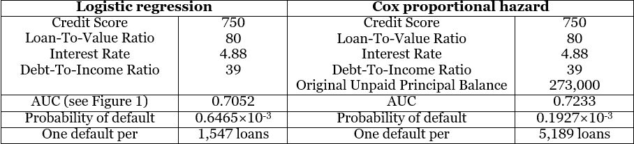
Below, Table 1 displays the outcomes of the optimal combination of variables that result in the highest AUC, along with the median values assigned to the model. Due to the strong skewness of most variables, median values are preferred over mean values. Additionally, the PD is provided, along with the calculation of the number of loans required to observe a single default. In this context, the Cox PH model estimates a lower PD in comparison to the logistic regression. While higher PD estimates are typically associated with greater costs, they also serve as an additional precautionary measure, for example in the event of a financial downturn.

In summary, the two proposed models represent only a minor selection of the numerous models available for capturing PD and credit risk. As the differences in default probabilities are significant, the models should be tested for consistency, alignment with underlying assumptions and overall robustness.

In general, this analysis highlights the importance of effective credit risk management and shows how financial institutions can estimate the probability of default and mitigate risk.

If you want to learn more about modeling credit risk, or our consulting services, let us contact you, or please feel free to contact the author of this article:

Max Bastiaens | m.bastiaens@vbadvisory.nl

References

• BCBS (2001, May 31). Consultative Document: The Internal Ratings-Based Approach.
• Supporting Document to the New Basel Capital Accord. https://www.bis.org/publ/bcbsca05.pdf
• Benmelech, E., & Dlugosz, J. (2010). The credit rating crisis. NBER macroeconomics annual, 24(1), 161-208.
• Cao, R., Vilar, J. M., & Devia, A. (2009). Modelling consumer credit risk via survival analysis. SORT: statistics and operations research transactions, 33(1), 0003-30.
• Cox, D. R. (1972). Regression models and life-tables. Journal of the Royal Statistical Society: Series B (Methodological), 34(2), 187-202.